We propose a novel paradigm to deal with depth reconstruction from 4D light fields. Our method offers both a fast purely local depth estimation within a light field structure, as well as the option to obtain very accurate estimates using a variational global optimization framework.
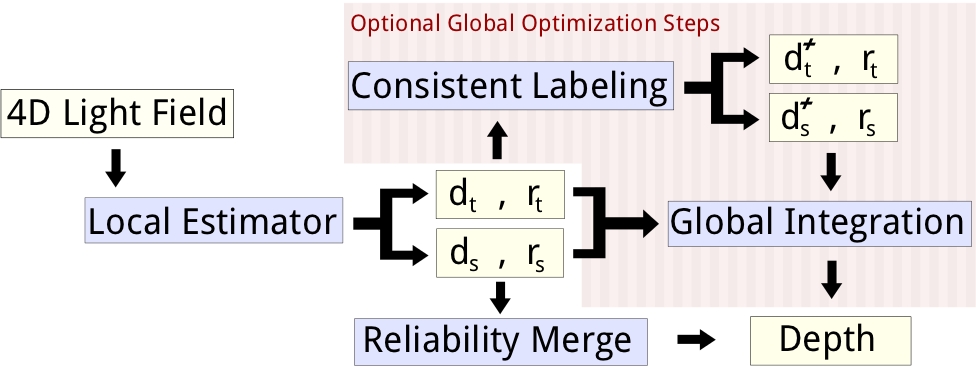
- The input is a 4D light field parameterized as a Lumigraph [1].
- The first step is a local depth labeling on 2D sections of the Lumigraph, so-called epipolar plane images (EPI)[2], described in
Local Depth Labeling in EPI Space. This results in two channels \(d_s,d_t\) with depth information and corresponding reliability estimates \(r_s,r_t\).
- Extracting the labels by comparing these reliabilities pixel-wise yields a 4D depth field. As an alternative to this simple reliability merge we also provide a (slower) global integration which produces a globally optimal solution to the depth map merging problem.
- An optional global optimization step also offers a Consistent EPI Depth Labeling, taking the inherent structure of epipolar plane images into account.
 |
 |
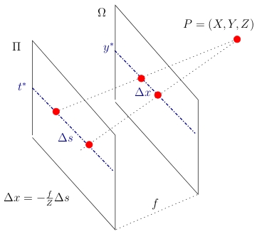
| Light field geometry |
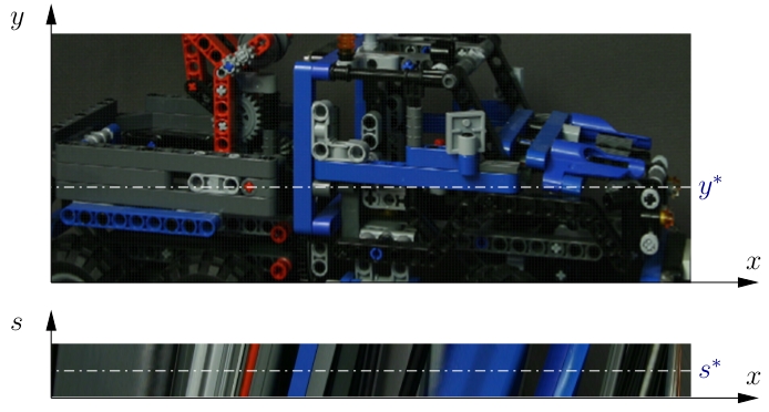
Pinhole view at \( (s^*,t^*) \) and epipolar plane image \( S_{y^*,t^*}\) |
Each camera location \( (s^*,t^*) \) in the image plane \( \Pi \) yields a different pinhole view of the scene. By fixing a horizontal line of constant \( y^* \) in the image plane and a constant camera coordinate \( t^* \), one obtains an epipolar plane image (EPI) in $(x,s)$ coordinates. A scene point \( P \) is projected onto a line in the EPI due to a linear correspondence between its \(s\)- and projected \(x\)-coordinate.
In order to obtain the local depth estimate, we need to estimate the direction of epipolar lines on the EPI. This is done using the structure tensor \(J\) of the epipolar plane image \(S=S_{y^*,t^*}\),
\[
J =
\left[
\begin{matrix}
G_\sigma\ast(S_x S_x) & G_\sigma\ast(S_x S_y) \\
G_\sigma\ast(S_x S_y) & G_\sigma\ast(S_y S_y)
\end{matrix}
\right]
=
\left[
\begin{matrix}
J_{xx} & J_{xy} \\
J_{xy} & J_{yy}
\end{matrix}
\right].
\]
Here, \(G_\sigma\) represents a Gaussian smoothing operator at an outer scale~$\sigma$ and \(S_x,S_y\) denote the gradient components of \(S\) calculated on an inner scale \(\tau\). The direction of the local level lines can then be computed via
\[n_{y^*,t^*} = \begin{bmatrix} J_{yy} - J_{xx}\\
2 J_{xy}
\end{bmatrix} = \begin{bmatrix} \Delta x \\ \Delta s \end{bmatrix},
\]
from which we derive the local depth estimate (from equation in figure 'Light field geometry') as
\[d_{y^*,t^*} = -f \frac{ \Delta s }{\Delta x }.\]
As a reliability measure we use the
coherence of the structure tensor,
\[r_{y^*,t^*} := \frac{\left( J_{yy} - J_{xx}\right)^2+ 4J_{xy}^2}{\left( J_{xx} + J_{yy}\right)^2}.\]
 |
 |
| Epipolar plane image |
Local depth labeling |
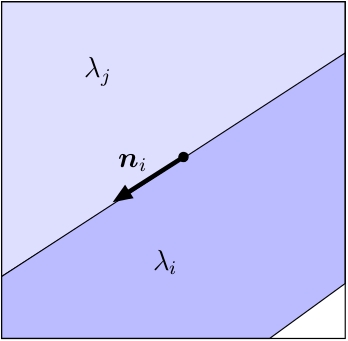
Each scene point projects to a line in the epi-polar-plane image, with a slope inversely proportional to the distance to the image plane. Because of occlusion ordering, a line labelled with depth \(\lambda_i\) corresponding to direction \(n_i\) cannot be crossed by a line with a dept \(\lambda_j > \lambda_i\), which is further away from the observer.
 |
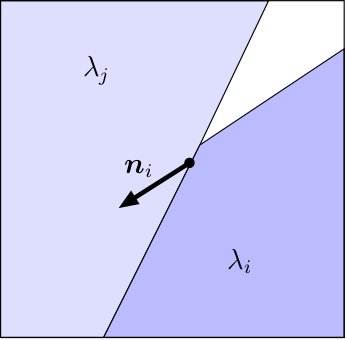 |
| Allowed if $\lambda_i
| Forbidden if $\lambda_i
|
We enforce these constraints by penalizing transitions from label \(\lambda_i\) to \(\lambda_j\) into direction \(\nu\) with
\[
p(\lambda_i, \lambda_j, \nu) := \begin{cases}
0 &\text{ if }i=j,\\
\infty &\text{ if } i [3], where the authors describe the construction of a regularizer \(R\) to enforce the desired ordering constraints. As a data term, we use the absolute distance between local estimate above and candidate label, since impulse noise is dominant.
|
 |
| Epipolar plane image |
Consistent depth labeling |
After obtaining EPI depth estimates \(d_{y^*,t^*}\) and \(d_{x^*,s^*}\) from the horizontal and vertical slices, respectively (either locally or from consistent depth labeling), we need to consolidate those estimates into a single depth map, which we obtain as the minimizer \(u\) of a global optimization problem.
- As a data term, we choose the minimum absolute difference to the respective local estimates weighted with the reliability estimates,
\[
\begin{aligned}
\rho(u,x,y) :=
\min( &r_{y^*,t^*}(x,s^*) | u - d_{y^*,t^*}(x,s^*) |, \\
&r_{x^*,s^*}(y,t^*) | u - d_{x^*,s^*}(y,t^*) | ).
\end{aligned}
\]
- As a regularizer, we choose total variation, since this allows us to compute globally optimal solutions to the functional using the technique of functional lifting described in [4].
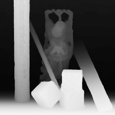
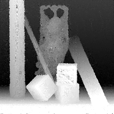
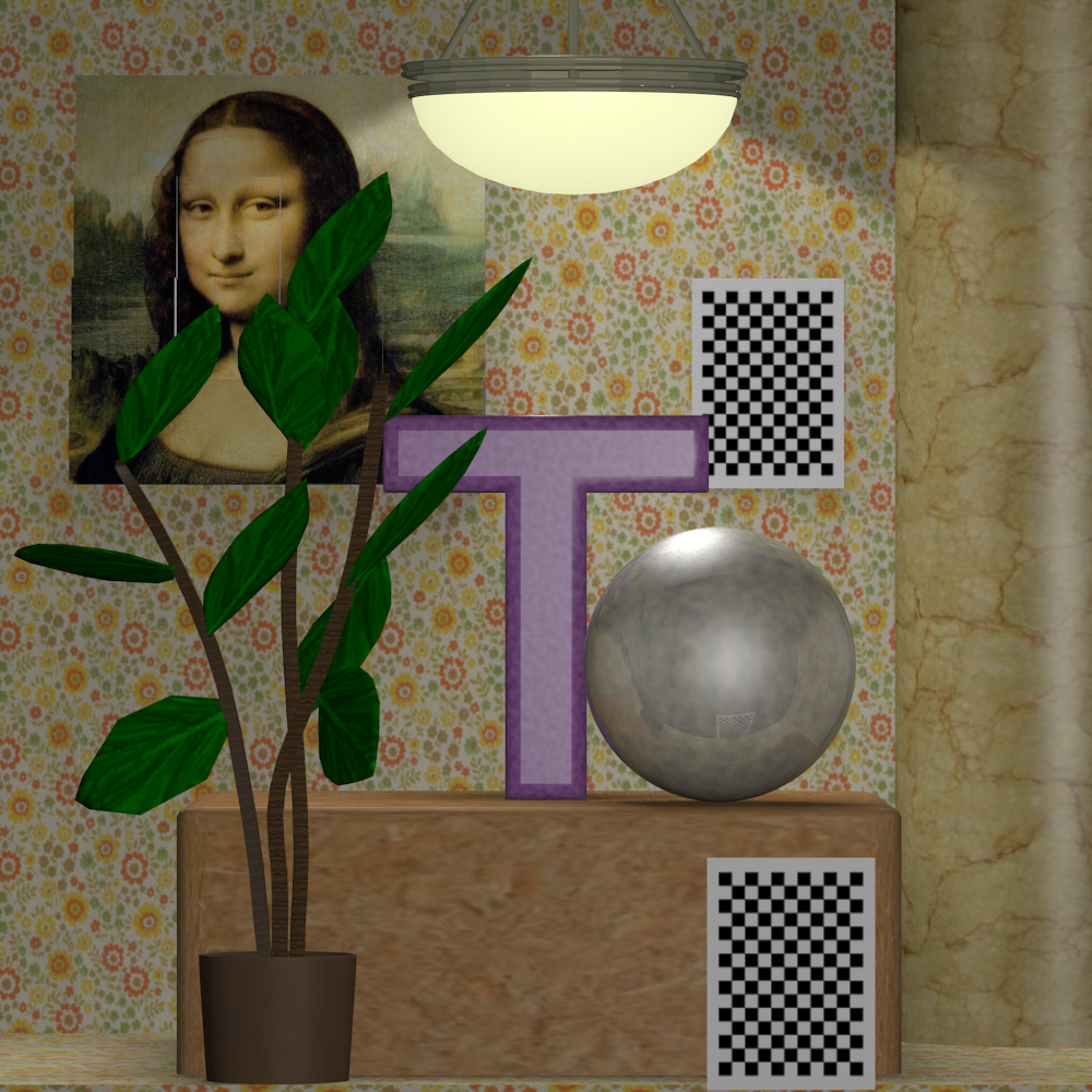
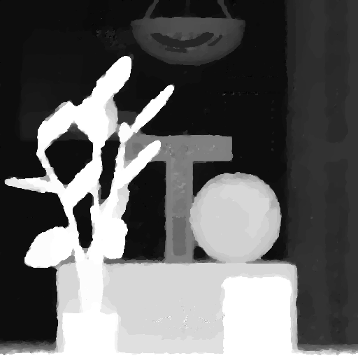
Results on synthetic light fields:
 |
 |
 |
 |
| Central View |
Local |
Global |
Consistent |
 |
 |
 |
 |
| Central View |
Local |
Global |
Consistent |
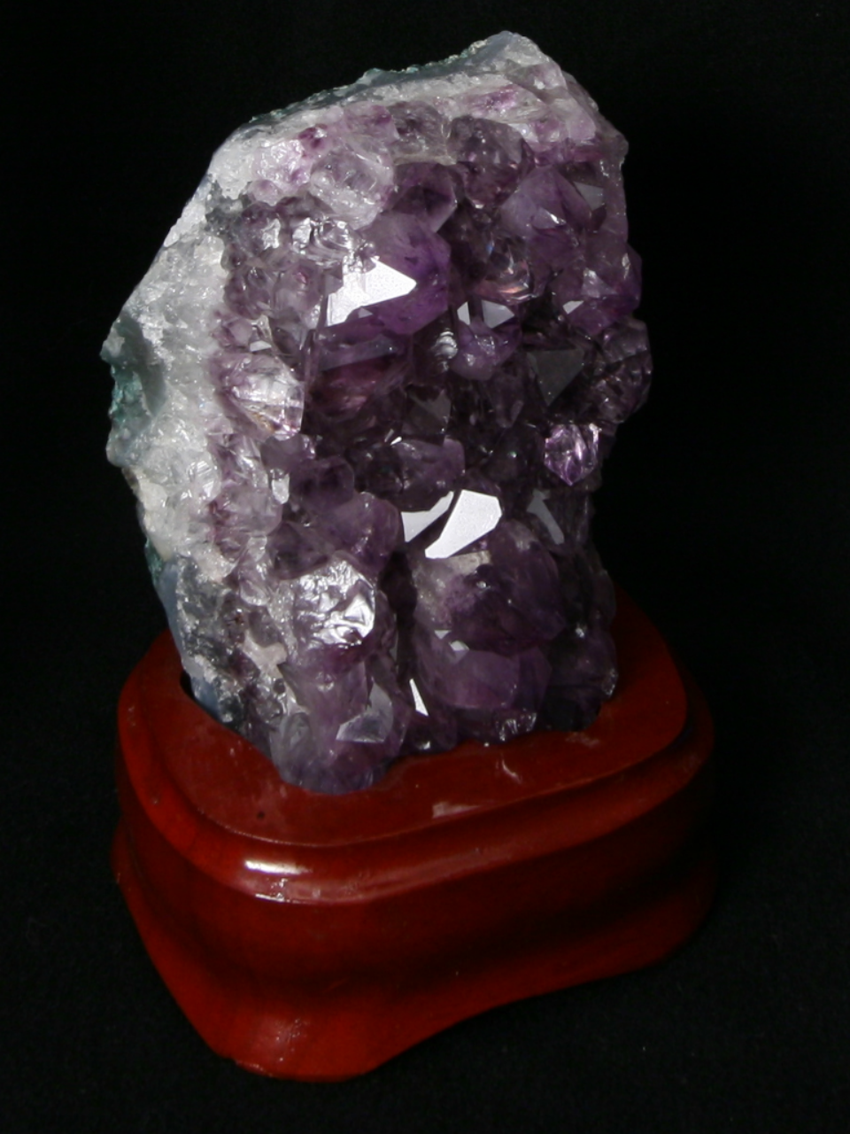
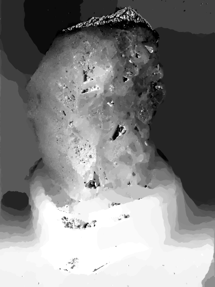
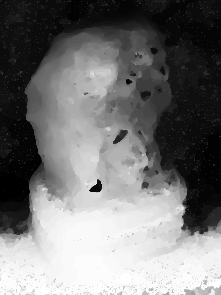
Results on stanford light fields:
 |
 |
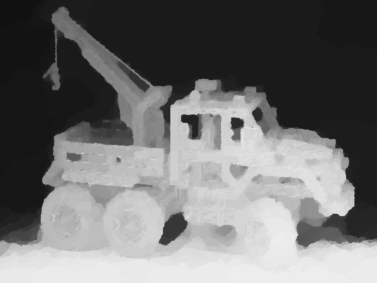 |
| Central View |
Stereo |
Global |
 |
 |
 |
| Central View |
Stereo |
Global |
Results on light fields from a plenoptic camera:
 |
 |
 |
| Central View |
Stereo |
Global |
|
 |
 |
| Central View |
Stereo |
Global |